How Shall We Play a Game? A Game-theoretical Model for Cyber-warfare Games Tiffany Bao∗, Yan Shoshitaishvili†, Ruoyu Wang†, Christopher Kruegel†, Giovanni Vigna†, David Brumley^{∗ ∗}Carnegie Mellon University {tiffanybao, dbrumley}@cmu.edu †UC Santa Barbara {yans, fish, chris, vigna}@cs.ucsb.edu Abstract—Automated techniques and tools for finding, exploiting and patching vulnerabilities are maturing. In order to achieve an end goal such as winning a cyber-battle, these techniques and tools must be wielded strategically. Currently, strategy development in cyber – even with automated tools – is done manually, and is a bottleneck in practice. In this paper, we apply game theory toward the augmentation of the human decision-making process. Our work makes two novel contributions. First, previous work is limited by strong assumptions regarding the number of actors, actions, and choices in cyber-warfare. We develop a novel model of cyber-warfare that is more comprehensive than previous work, removing these limitations in the process. Second, we present an algorithm for calculating the optimal strategy of the players in our model. We show that our model is capable of finding better solutions than previous work within seconds, making computertime strategic reasoning a reality. We also provide new insights, compared to previous models, on the impact of optimal strategies. I. INTRODUCTION In recent years, security researchers have pursued automated vulnerability detection and remediation techniques, attempting to scale such analyses beyond the limitations of human hackers. Eventually, automated systems will be heavily, and maybe predominantly, involved in the identification, exploitation, and repair of software vulnerabilities. This will eliminate the bottleneck that human effort represented in these areas. However, the human bottleneck (and human fallibility) will remain in the higher-level strategy of what to do with automatically identified vulnerabilities, automatically created exploits, and automatically generated patches. There are many choices to make regarding the specificities of such a strategy, and these choices have real implications beyond cyber-security exercises. For example, nations have begun to make decisions on whether to disclose new software vulnerabilities (zero-day vulnerabilities) or to exploit them for gain [17, 36]. The NSA recently stated that 91% of all zero-days it discovers are disclosed, but only after a deliberation process that carefully weighs the opportunity cost from disclosing and finally forgoes using a zero-day [28]. Before disclosure, analysts at the NSA manually consider several aspects, including the potential risk to national security if the vulnerability is unpatched, the likelihood of someone else exploiting the vulnerability, and the likelihood that someone will re-discover the vulnerability [11]. In this paper, we explore the research question of augmenting this human decision-making process with automated techniques rooted in game theory. Specifically, we attempt to identify the best strategy for the use of an identified zero-day vulnerability in a "cyber-warfare" scenario where any action may reveal information to adversaries. To do this, we create a game model where each new vulnerability is an event and "players" make strategic choices in order to optimize game outcomes. We develop our insight into optimal strategies by leveraging formal game theory methodology to create a novel approach that can calculate the best strategy for all players by computing a Nash equilibrium. Prior work in the game theory of cyber warfare has serious limitations, placing limits on the maximum number of players, requiring perfect information awareness for all parties, or only supporting a single action on a single "event" for each player throughout the duration of the entire game. As we discuss in Section II-B, these limitations are too restrictive for the models to be applicable to real-world cyber-warfare scenarios. Our approach addresses these limitations by developing a multi-round game-theoretic model that accounts for attack and defense in an imperfect information setting. Technically, our game model is a partial observation stochastic game (POSG) where games are played in rounds and players are uncertain about whether other players have discovered a zeroday vulnerability. Additionally, our model supports the concept of sequences of player actions. Specifically, we make two new observations and add support for them to our model. First, attacks launched by a player can be observed and reverse-engineered by that player's opponents, a phenomenon we term "attack ricocheting" [4]. Second, patches created by a player can be reverse-engineered by their opponents to identify the vulnerability that they were meant to fix, a concept called "automated patch-based exploit generation" (APEG) in the literature [6]. This knowledge, in turn, can be used to create vulnerabilities to attack other players. A central challenge in our work was to develop an approach for computing the Nash equilibrium of such a game. A Nash equilibrium is a strategy profile in which none of the players will have more to gain by changing the strategy. It characterizes the stable point of the game interaction in which all players are rationally playing their best responses. However, computing a Nash equilibrium is known as a Polynomial Parity Argument on Directed Graphs-complete (PPAD-complete) problem [14], 2017 IEEE 30th Computer Security Foundations Symposium © 2017, Tiffany Bao. Under license to IEEE. DOI 10.1109/CSF.2017.34 7

which is believed to be hard. We overcome this problem in our context by taking advantage of specific characteristics of cyber-warfare games, allowing us to split the problem of computing the Nash equilibrium into two sub-problems, one of which can be converted into a Markov decision process problem and the other into a stochastic game. Our algorithm is able to compute the Nash equilibrium in polynomial time, guaranteeing the tool's applicability to real-world scenarios. Using the new model and the new algorithm, our tool finds better strategies than previous work [25, 31]. Contrary to previous work, we find that players have strategies with more utility than to attack or to disclose all the time throughout the game. Specifically, we find that in some situations, depending on various game factors, a player is better served by a patch-then-attack strategy (e.g., the NSA could disclose the vulnerability, patch their software, and then still attack) or by a pure disclose strategy (see § VI). These are new results not predicted by previous models. Our tool not only found the order of the actions, but also provided a concrete plan for actions over rounds, such as "patch, then attack after 2 rounds of patching". Moreover, we observe that a previous result of prior work in the area – the concept that it is always optimal for at least one player to attack – does not stand in our expanded model (see § VI). We demonstrated this by showing an example where the optimal strategy for both players is to disclose and patch. We also observe that a player must ricochet and patch fast enough in order to prevent his opponent from attacking and forcing the vulnerability disclosure. If a player is only able to either ricochet or patch fast enough, they might still get attacked. The optimal strategies derived from our models have realworld consequences – in a case study in this paper, we apply our model to a recent fully-automated cyber security contest run by DARPA, the Cyber Grand Challenge, which had 4.25 million dollars in prizes. Our study shows that an adoption of our model by the third-place team, team Shellphish, would have heavily improved their final standing. The specific strategy picked in the approach to cyber warfare matters, and these choices have real-world consequences. In the CGC case, the consequence was a difference of prize winnings, but in the real world (the challenges of which the CGC was designed to mirror [12]), the difference could be more fundamental. Overall, this paper makes the following contributions: • We develop a novel model of cyber-warfare that is more comprehensive than previous work because it 1) considers strategies as a sequence of actions over time, 2) addresses players' uncertainty about their opponents, and 3) accounts for more offensive and defensive techniques that can be employed for cyber-warfare, such as ricocheting and APEG (Section III). • We present an algorithm for calculating the optimal strategy of the players in our model. The original model is a POSG game, which, in general, is intractable to solve [23]. We take advantage of the structure of cyber-warfare and propose a novel approach for finding the Nash equilibrium (Section IV). • We show that our model is capable of finding better solutions than previous work within seconds. We also provide new insights, compared to previous models, on the impact of optimal strategies. We demonstrate that optimal strategies in a cyber-warfare are more complex than previous conclusions [25, 31], and one must take into consideration the unique aspect of cyber-warfare (versus physical war), i.e., that exploits can be generated by the ricochet and APEG techniques. This insight leads to new equilibriums not predicted by previous work [25, 31] (Section VI). II. BACKGROUND In this section, we review the concepts that are relevant to our cyber security model. Furthermore, we present an in-depth discussion of existing work in game-theoretical modeling of cyber warfare. An in-depth understanding of game theory is not required for an overall understanding of our work, and we do not include a dedicated discussion on game theory. For the dedicated reader, there are many excellent game theory resources that can provide a deep understanding [20, 33]. A. Game Models & Nash Equilibriums Game-theoretic approaches cover a range of game models, depending on the game in question. We show the relationship of game models in Figure 1. In cyber security games, players hide information about their exploit development. To accommodate this, we set up the model as an incomplete information game where the players in the model do not know whether other players have discovered a zero-day or not. This assumption is natural: an exploit is only a zero-day from the perspective of each player having never seen it before. Because cyber security games last from hours to days, it is possible for players to take multiple actions in a game. For example, a player could hold a vulnerability at the beginning of the cyber security game and exploit other players later. In order to support these strategies, we design our model as a multi-stage game. Furthermore, the players may find a vulnerability at any time during the game, changing the state of the game from that point. This property is supported by the concept of a stochastic game (SG). For an SG, the game played at any given iteration depends probabilistically on the previous round played and the actions of players in previous round. SG can also be viewed as a multi-player version of Markov Decision Process (MDP) [15]. Combining these concepts, if a game 1) has players with incomplete information, 2) consists of multiple rounds, and 3) players' knowledge may change during the game, then the game is a partially observable, stochastic game (POSG). A POSG can also be considered as a multi-player equivalent of a partially observable Markov decision process (POMDP). A Nash equilibrium is a strategy profile in which players will not have more to gain by changing their strategy. In our paper, we will focus on building the game model and finding the Nash 8

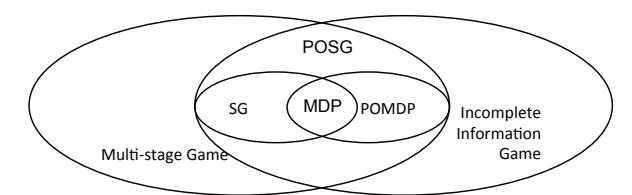
POSG MDP - Fig. 1: The relationship of game models. equilibrium of the game. Although there are cases of games calling for significantly more refined equilibrium concepts (e.g., perfect Bayesian equilibrium or sequential equilibrium), we follow the argument from previous work, which claims that the generally-coarser concept of Nash equilibrium adequately captures the strategic aspects of cyber security games [25]. B. Game Theory of Cyber Warfare Game theory has been applied in many security contexts, most commonly with a focus on network security or the economics of security, e.g., [1, 7, 8, 16, 21, 22, 24, 26, 29, 35]. In our paper, we focus exclusively on game theory as it is applied specifically to cyber-warfare situations. In this section, we will describe existing approaches to modeling cyber-warfare and discuss our improvements over these techniques. Moore et al. [25] proposed the cyber-hawk model in order to find the optimal strategy for both players. The cyber-hawk model describes a game where each player chooses to either keep vulnerabilities private (and create exploits to attack their opponent) or disclose them. They conclude that the first player to discover the vulnerability should always attack, precluding vulnerability disclosure. However, this model is limited to a one-shot game where players are only allowed to make one choice between attack and disclosure. After this choice, the game is over. This limitation makes the approach an unrealistic one for modeling real-life cyber-warfare. The cyber-hawk model raised new questions that need to be explored, such as if a player determines to use a vulnerability offensively, how soon they should commence the attack. Schramm [31] proposes a dynamic model to answer this question. The model indicates that waiting reduces a player's chance of winning the game, which implies that if a player determines to attack, he should act as soon as possible. The Schramm model relies on a key assumption of full player awareness, requiring that players know whether, and how long ago, their opponent discovered a vulnerability. This assumption is unlikely to be valid in real-world scenarios, because nations keep the retained vulnerabilities (if they have any at all) secret. Additionally, it is still limited to two players and supports only one single taken action, after which the game ends. Given the latest defensive and offensive techniques [2, 4, 34] and the evaluation on the impacts of zero-day attacks [5, 19], we observe three things missing in previous models that are vital for choosing players' best strategies in cyber-warfare. First, players in a cyber-warfare often have multiple actions over multiple rounds. As an example of a multiple round game, consider the NSA statement above. Although the NSA claimed to disclose 91% of all zero-day vulnerabilities, it did not mention whether they ever exploited (even if just a single machine) before or after the disclosure. Second, players in cyber-warfare are uncertain whether other players have discovered vulnerabilities. Instead, players use observations such as network traffic and patch releases to infer possible states. This uncertainty influences player decisions, as a player must account for all the possible states of the other players in order to maximize his expected utility. Previous approaches cannot be extended to handle multiple steps with partial information and dependencies. Third, both attacking and disclosing reveal the information of a vulnerability. Previous work showed that a patch may be utilized by attackers to generate new exploits [6]. However, we show that attacking leaks information, and we introduce the notion of ricochet into the game theory model. In the automated patch-based exploit generation (APEG) [6] technique, a player infers the vulnerable program point from analyzing a patch and then creates an exploit. Similarly, in the ricochet attack technique, a player detects an exploit (e.g., through network monitoring or dynamic analysis) and then turns around and uses the exploit against other players. For instance, Costa et al. have proposed monitoring individual programs to detect exploits, and then replaying them as part of their technique for self-certifying filters [9], where the filters self-certify by essentially including a version of the original exploit for replay. Since then, fully-automated shellcode replacement techniques have emerged, making automatic exploit modification and reuse possible [4]. Both inadvertent disclosures (through attacks) and intentional disclosures (and patching) create new game actions which previous work does not account for. Policy makers and other users of previous models [25, 31] can reach incorrect conclusions and ultimately choose suboptimal strategies. III. PROBLEM STATEMENT AND GOALS In this section, we formally state the cyber-warfare game. We will describe the problem setup, lay out our assumptions, present the formalized POSG model and finally clarify the goal of our work. A. Problem Setup The cyber-warfare game needs to be general and compatible with known cyber-warfare events such as the Stuxnet event. One requirement is that the cyber-warfare game model must support players with comprehensive techniques, rather than the simple choices that prior models allow. Figure 2 shows the workflow of the player in our model. There are three ways for a player to learn of a vulnerability. A player may detect an attack, receive the disclosure from other players, or discover the vulnerability by himself. After a player learns a vulnerability, the strategy generator will compute the strategy for the vulnerability. 1) Players All players are participating in a networked scenario. They are capable of finding new vulnerabilities, monitoring their own 9

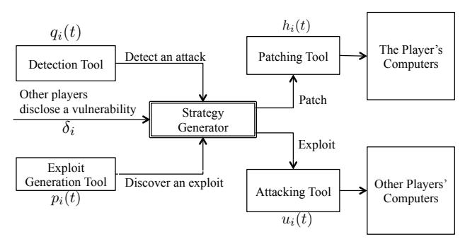
Attacking Tool Patching Tool Strategy Generator Exploit Generation Tool Detection Tool Other Players' Computers The Player's Computers Detect an attack Discover an exploit Patch Exploit Other players disclose a vulnerability qi(t) pi(t) hi(t) ui(t) δi Fig. 2: The workflow of the player in the cyber-warfare game. Parameter Definition ^pi(t) The probability distribution over time that player i discovers a vulnerability at round t. qi(t) The probability to launch a ricochet attack with exploits that player i received in the previous round. hi(t) The ratio of the amount of patched vulnerable resources over the total amount of vulnerable resources by t rounds after the vulnerability is disclosed. δi The number of rounds required by player i to generate a patch-based exploit after a vulnerability and the corresponding patch are disclosed. ^ui(t) The dynamic utility that player ⁱ gains by attacking his opponents at round t. TABLE I: Parameters for player i. connections and ricocheting an attack, patching after vulnerability disclosure, and generating patch-based exploits. Players may have different levels of skills, which are characterized using the parameters listed in Table I. These parameters are a substantial component of our model. For player i, the vulnerability discovery skill is denoted by pi(t), which is a function of probability that the player discovers a zero-day vulnerability distributed over rounds. Their level of ricochet ability is characterized by parameter qi(t), which is the probability of launching a ricochet attack with exploits they recovered from the traffic received in the previous round. A player's patching skill is represented by function hi(t). hi(t) is the ratio of the amount of patched vulnerable resources over the total amount of vulnerable resources by t rounds after the vulnerability is disclosed. In the real world, while patching a single computer might take only minutes, patching all vulnerable resources (depending on the organization, containing thousands of instances) might take days to months [5]. While one player is patching, other players could possibly attack, and any vulnerable resources that have not been patched will suffer from the attack. The last parameter, δi, describes player i's level of APEG skills, which is the number of rounds required by the player to generate a patch-based exploit after a vulnerability and the corresponding patch are disclosed. Finally, the attacking utility, denoted as ui(t), encodes the dynamic utility that player i gains by attacking his opponents at round t before the patch is released. 2) Player States and Actions Each player i has a state denoted by θⁱ in each round, where θⁱ ∈ Θⁱ = {¬D, D}. ¬D refers to the situation in which a player has not yet learned of a zero-day, while D refers to the situation in which a player knows the vulnerability, either by actively finding the vulnerability and developing an exploit or by passively "stealing" the exploit from an attack or a patch. In each round, players choose one of the following actions: {ATTACK, PATCH, NOP (no action), STOCKPILE}, where the semantics of ATTACK, PATCH, and NOP have their literal meaning, and STOCKPILE means holding a zero-day vulnerability for future use. Players are limited in their actions by their state. This is acceptable for stochastic games and does not impact the difficulty or insights of the model [20, §6.3.1]. In particular, while a player in state ¬D can only act NOP, a player in state D can choose an action among ATTACK, PATCH and STOCKPILE before the patch is released, and between ATTACK and NOP after the release, depending on their skill at detecting attacks or APEG. B. Game Factors & Assumptions Our model considers the game within the scope of the following factors and assumptions: • We do not distinguish between a player discovering the vulnerability and knowing about how to exploit it in our game. This is because in many cases, when a nation acquires a zero-day vulnerability, the nation also learns about the zero-day exploit. For example, nations acquire zero-day vulnerabilities by purchasing zero-day exploits from vulnerability markets [17, 18, 27]. We acknowledge that discovering a vulnerability and creating an exploit are conceptually different, but we leave the separation of those two as future work. • We do not distinguish between a player disclosing a vulnerability and releasing a patch. The known patching mechanisms such as Microsoft update make secret patching unlikely to happen in the real world, and in most cases, the disclosure of a vulnerability comes with a patch or a workaround. • We assume that players are monitoring their systems, and may probabilistically detect an attack. We also assume they may be able to then ricochet the exploit to other players. We note that the detection may come through monitoring of the network (in the case of network attacks), or other measures such as honeypots, dynamic analysis of suspicious inputs, etc. For example, Vigilante [9] detects exploits and creates a self-certifying alert (SCA), which is essentially a replayable exploit. We note that such attacks may be detected over a network (e.g., in CTF competitions, these are called reflection attacks [30]) or via dynamic analysis, as with Vigilante. • We assume that once a patch reveals information about the vulnerability, other players can use the patch to create an exploit. For example, Brumley et al. shows this can be done automatically in some instances [6]. We note that patch-based 10

t, ∅, ¬D, ¬D NOP, NOP t + 1, ∅, D, D t + 1, ∅, ¬D, D t + 1, ∅, D, ¬D t + 1, ∅, ¬D, ¬D p1(t)p2(t) (1 − p1(t))p2(t) p1(t)(1 − p2(t)) (1 − p1(t))(1 − p2(t)) (a) Neither player has discovered a vulnerability. t, ∅, ¬D, D t + 1, t, ¬D, D t + 1, ∅, ¬D, D t + 1, ∅, D, D t + 1, ∅, D, D t + 1, ∅, ¬D, D NOP, ATTACK NOP, STOCKPILE NOP, PATCH ¹ (1 − p1(t)) p1(t) q1(t) + p1(t)(1 − q1(t)) (1 − p1(t))(1 − q1(t)) (b) One player (player 2) has discovered a vulnerability. t, ∅, D, D PATCH, ∗ ∗, PATCH ATTACK, STOCKPILE ATTACK, ATTACK STOCKPILE, STOCKPILE STOCKPILE, ATTACK t + 1, ∅, D, D t + 1, t, D, D 1 1 (c) Both players have discovered and withhold the vulnerability. t, r, D, ¬D t, t − δ2, D, ¬D NOP, NOP ATTACK, NOP ∗, ∗ t + 1, r, D, D t + 1, r, D, ¬D t + 1, r, D, ¬D t + 1, t − δ2, D, D q2(t) 1 − q2(t) 1 1 (d) One player (player 1) has discovered and disclosed a vulnerability, while the other player has not discovered the vulnerability. t, r, D, D ATTACK, NOP ATTACK, ATTACK NOP, NOP NOP, ATTACK ^t + 1, r, ^D, ^{D 1} (e) Both players have discovered the vulnerability, and the vulnerability has been disclosed. Fig. 3: The transitions of game states. For each sub-figure, the left-hand side is the state of the current round and the right-hand side is the state of the next round. NOT DISCOVER DISCOVER NOP ATTACK STOCKPILE PATCH NOT DISCOVER NOP 0 −u2(t) 0 0 DISCOVER ATTACK u1(t) u1(t) − u2(t) u1(t) 0 STOCKPILE 0 −u2(t) 0 0 PATCH 0 0 00 TABLE II: The reward matrix at round t before patch is released. The table shows the reward of player 1 (the row player). The reward of player 2 (the column player) is the negative value of that of player 1. skill level. This is because the probability is inferred based on players' attributes, such as the discovery probability, ricochet probability, and those attributes are public to all players. Finally, although players are uncertain about the state of the other players (which they represent as a probability distribution of player states), they know the probability of their opponents being in a state given the public information of the opponents, such as the vulnerability discovery probability (e.g., based upon prior zero-day battles) and the ricochet probability. Based on the above insights, we convert the POSG model to a stochastic game model by encoding the belief of each player into the game state. In our game, the belief of a player is the probability that the player thinks the other player has found the vulnerability. We can compute the Nash equilibrium for the converted stochastic game by dynamic programming. We will also discuss the observation of players' strategy after vulnerability disclosure. A. The Stochastic Game As our assumption that a player's belief about the state of opponent players can be estimated from the globally-known player properties, the POSG model reduces to a much more tractable stochastic model in the pre-disclosure phase. We define the stochastic game (SG) model SG = N ^S, A^S, Θ^S, Φ^S, R^S We retain the definition of players in POSG, N ^P = N ^S = {player 1, player 2}. 1) Player Actions The player action in SG is defined as a combination of player actions under different player states. For example, if 12

NOT DISCOVER DISCOVER NOP ATTACK NOP DISCOVER NOP 0 −u2(t)h1(t − r) 0 ATTACK u1(t)h2(t − r) u1(t)h2(t − r) − u2(t)h1(t − r) u1(t)h2(t − r) NOT DISCOVER NOP 0 −u2(t)h1(t − r) 0 TABLE III: The reward matrix at round t after patch is released. The table shows the reward of player 1 (the row player). The reward of player 2 (the column player) is the negative value of that of player 1. player i plays ATTACK in state D and NOP in state ¬D, the corresponding action in the SG model is {D : ATTACK, ¬D : NOP}. For each player action ai, we will use ai[D] and ai[¬D] to denote the action in state D and ¬D, respectively. 2) Game State The game state Θ^S in the SG model is defined as Θ^S = T × R ×R×R. Besides the current round number T and the patch releasing round number R, a game state includes the beliefs of the two players about each other, which is the probability that a player has discovered a vulnerability from the other player's perspective, bⁱ ∈ [0, 1]. A game state θ^S ∈ Θ^S can be represented as θ^S = t, r, b1, b2, in which player 2 thinks the probability that player 1 has discovered the vulnerability is b1, and player 1 thinks the probability that player 2 has discovered the vulnerability is b2. Unlike the POSG model, the game states in the SG model include the uncertainty of a player about the other player's state. In each round of the game, players know their own states; although they do not know the other player's state, they infer the likelihood of the other player's state based on the other player's parameters. In addition, a player also knows the other player's beliefs about the game state because the player also knows the parameters of himself. Therefore, we are able to convert to the SG model under the structure of the game states above. 3) State Transition We define the state transition function of the SG model as Φ^S : Θ^S × A^{S 1} × A^{S 2} → Δ(Θ^S). We represent the probability that a game transitions to θ^S using Φ^S(·)[θ^S]. The transition between the game states is shown in Figure 4. The game states are divided by the time before and after vulnerability disclosure, because the actions and information available to players are different between the two phases. Before Disclosure (Figure 4a). Suppose the game is in state t, ∅, b1, b2. If neither player acts ATTACK, the probability that player i discovers the exploits at the current round is pi(t) and the probability that player i discovers the exploit by the current round is 1 − (1 − bi)(1 − pi(t)). The game transits to state t+ 1, ∅, 1−(1−b1)(1−p1(t)), 1−(1−b2)(1−p2(t)). If a player chooses to ATTACK, the probability that their opponent will acquire the exploit in the current round is the joint probability that the opponent discovers the vulnerability by himself and that he detects the exploit. Meanwhile, if the opponent detects the exploit, they will be certain that the attacker has the exploit. For example, if player 1 's action is {D : ATTACK, ¬D : NOP} while player 2 's action is {D : STOCKPILE, ¬D : NOP}, the game will transition to t+1, ∅, 1−(1−b1)(1−p1(t)), 1−(1−b2)(1−p2(t))(1−q2(t)) with the probability of 1−q2(t) and t+1, ∅, 1, 1−(1−b2)(1− p2(t))(1 − q2(t)) with the probability of q2(t). Similarly, if both players act ATTACK in state D, the game will transition to one of four possibilities. If neither player detects the exploit, the game state will be t + 1, ∅, 1 − (1 − b1)(1−p1(t))(1−q1(t)), 1−(1−b2)(1−p2(t))(1−q2(t)). If player 1 detects the exploit while player 2 does not, the game state will be t + 1, ∅, 1 − (1 − b1)(1 − p1(t))(1 − q1(t)), 1. If player 2 detects the exploit while player 1 does not, the game state will be t + 1, ∅, 1, 1 − (1 − b2)(1 − p2(t))(1 − q2(t)). Finally, if both players detect the exploit, the game state will be t + 1, ∅, 1, 1. If one player acts PATCH, both players will patch immediately. If player 1 releases a patch, the game will transition to t + 1, t, 1, b2, as everyone is certain that player 1 has the exploit. If player 2 releases a patch, the game will transit to t+1, t, b1, 1 and if both player release a patch, the game will transition to t + 1, t, 1, 1. After Disclosure (Figure 4b). After disclosure, both players will know the vulnerability so they will stop searching for it. Also, the player disclosing a vulnerability is public so both players know that the player is in state D. Suppose player 1 discloses a vulnerability in round r. In response, player 2 starts APEG and will generate the exploit by round r + δ2. Meanwhile, player 2 still has the chance to ricochet attacks if player 1 attacks. Therefore, the belief of player 2 's possession of the exploit will increase if player 1 attacks in the previous round. 4) Utility We calculate players' utility by the single-round reward function R^S : Θ^S × A^{S 1} × A^{S 2} → R. Given a game state and players actions, the single-round reward is equal to the expected reward over player states. Given player i and a player state θi, the probability that the player is in state θⁱ when the SG game state is θ^S = t, r, b1, b2, which is denoted by P(θ^S, θi), is equal to ^P(θ^S, θi) = ^P(t, r, b1, b2, θi) = bⁱ if θⁱ = ¬D 1 − bⁱ if θⁱ = D Recall the reward function for the POSG model R^P : A^{P 1} × A^{P 2} → R takes as input the players' actual actions and produces as output the utility of one player (because the utility of the other is the negative value for zero-sum game). We calculate the reward for the SG model using R^P . In specific, we have RS(θS, a^{S 1} , a^{S 2} ) = θ1 θ2 P(θS, θ1)P(θS, θ2)R^P (a^{S 1} [θ1], a^{S 2} [θ2]) 13

t, ∅, b1, b2 {D : PATCH, ¬D : NOP},{D : PATCH, ¬D : NOP} {D : PATCH, ¬D : NOP},{D : ATTACK, ¬D : NOP} {D : PATCH, ¬D : NOP},{D : STOCKPILE, ¬D : NOP} {D : ATTACK, ¬D : NOP},{D : PATCH, ¬D : NOP} {D : STOCKPILE, ¬D : NOP},{D : PATCH, ¬D : NOP} {D : ATTACK, ¬D : NOP},{D : ATTACK, ¬D : NOP} {D : ATTACK, ¬D : NOP},{D : STOCKPILE, ¬D : NOP} {D : STOCKPILE, ¬D : NOP},{D : ATTACK, ¬D : NOP} {D : STOCKPILE, ¬D : NOP},{D : STOCKPILE, ¬D : NOP} t + 1, t, 1, 1 t + 1, t, 1, 1 − (1 − b2)(1 − p2(t)) t + 1, t, 1, 1 t + 1, t, 1, 1 − (1 − b2)(1 − p2(t)) t + 1, t, 1 − (1 − b1)(1 − p1(t)), 1 t + 1, t, 1, 1 t + 1, t, 1 − (1 − b1)(1 − p1(t)), 1 t + 1, ∅, 1 − (1 − b1)(1 − p1(t))(1 − q1(t)), 1 t + 1, ∅, 1, 1 − (1 − b2)(1 − p2(t))(1 − q2(t)) t + 1, ∅, 1, 1 t + 1, ∅, 1 − (1 − b1)(1 − p1(t))(1 − q1(t)), 1 − (1 − b2)(1 − p2(t))(1 − q2(t)) t + 1, ∅, 1 − (1 − b1)(1 − p1(t)), 1 − (1 − b2)(1 − p2(t))(1 − q2(t)) t + 1, ∅, 1, 1 − (1 − b2)(1 − p2(t))(1 − q2(t)) t + 1, ∅, 1 − (1 − b1)(1 − p1(t))(1 − q1(t)), 1 − (1 − b2)(1 − p2(t)) t + 1, ∅, 1 − (1 − b1)(1 − p1(t))(1 − q1(t)), 1 t + 1, ∅, 1 − (1 − b1)(1 − p1(t)), 1 − (1 − b2)(1 − p2(t)) 1 1 − q1(t) q1(t) 1 1 − q2(t) q2(t) 1 q1(t)(1 − q2(t)) (1 − q1(t))q2(t) q1(t)q2(t) (1 − q1(t))(1 − q2(t)) 1 − q2(t) q2(t) 1 − q1(t) q1(t) 1 (a) Before disclosing a vulnerability. t, r, 1, b2 {D : ATTACK},{D : ATTACK, ¬D : NOP} {D : ATTACK},{D : STOCKPILE, ¬D : NOP} {D : STOCKPILE},{D : ATTACK, ¬D : NOP} {D : STOCKPILE},{D : STOCKPILE, ¬D : NOP} t + 1, r, 1, b² + (1 − b2)q2(t) t + 1, r, 1, 1 t + 1, r, 1, b² + (1 − b2)q2(t) t + 1, r, 1, b2 t + 1, r, 1, 1 t + 1, r, 1, b2 t, t − δ2, 1, b2 {D : ATTACK},{D : ATTACK, ¬D : NOP} {D : ATTACK},{D : STOCKPILE, ¬D : NOP} {D : STOCKPILE},{D : ATTACK, ¬D : NOP} {D : STOCKPILE},{D : STOCKPILE, ¬D : NOP} t + 1, t − δ2, 1, 1 1 − q1(t) q1(t) 1 1 − q1(t) q1(t) 1 1 (b) After disclosing a vulnerability. Suppose player 1 discloses a vulnerability. Fig. 4: The transition of game states in the stochastic game. The left-hand sides of the arrows are game states with possible strategies. The right-hand sides of the arrows are the possible game states after transition. B. Compute the Nash Equilibrium A Nash equilibrium is a strategy profile where neither player has more to gain by altering its strategy. It is the stable point of the game when both players are rational and making their best response. Let NE^S : Θ^S → R denote player 1 's utility when both players play the Nash equilibrium strategy in the SG model. Since the game is a zero-sum game, the utility of player 2 is equal to −NE^S. We compute the Nash equilibrium inspired by the Shapley method [32], which is a dynamic programming approach for finding players' best responses. For game state θ^s = t, r, b1, b2, the utility of player 1 is equal to sum of the reward that player 1 gets in the current round and the expected utility that he gets in the future rounds. In the future rounds, players will continue to play with their best strategies, so the utility in the future rounds is equal to the one that corresponds to the Nash equilibrium in the future game states. Therefore, the utility of the Nash equilibrium of a game state is as following: NES(θS) = max a^{S 1} ∈A^S min a^{S 2} ∈A^S RS(θS, a^{S 1} , a^{S 2} )+ θ∈ΘS ΦS(θS, a^{S 1} , a^{S 2} )[θ] · NES(θ) (1) 14

In theory, the game could go for infinite rounds when neither players discloses a vulnerability. In this case, the corresponding utility will be equal to 0, positive infinity or negative infinity. However, for implementation, we need to set a boundary to guarantee that the recursive calculation of Nash equilibrium will stop. We introduce MAX^t to denote the maximum round of the game, and we assume that NES(t, r, b1, b2)=0, if t ≥ MAXt. (2) C. Optimize the Game After Disclosure Equation 1 is only applicable for calculating the Nash equilibrium of the SG model. Nonetheless, we find an optimized way to compute the Nash equilibrium after the vulnerability is disclosed (r = ∅). The optimized approach is based on the finding that if a player discloses a vulnerability, the other player should attack right after he generates the exploits. We call the player who discloses the vulnerability the explorer, and the other player who witness the disclosure of the vulnerability the observer. Intuitively, disclosure implies that the explorer has discovered the vulnerability, and the observer's attack will not reveal to the explorer any new information about the vulnerability. Therefore, there is no collateral damage if the observer attacks, and the observer's best strategy is to constantly attack until his adversary completes patching. We formally prove the finding as follows. Theorem 1. If one player discloses a vulnerability, the best response of the other player is {D : ATTACK, ¬D : NOP}. Proof. Without loss of generality, we assume that player 1 discloses a vulnerability, and the current game state for the SG model is SGt, r, 1, b2. The corresponding game state for the POSG model is either POSGt, r, D, D or POSGt, r, D, ¬D, shown in Figure 5. If player 2 has not discovered the vulnerability, then the actual game state is POSGt, r, D, ¬D. Player 2 can only play NOP, so their action is NOP when they are in state ¬D. If player 2 has discovered the vulnerability, then the actual game state is POSGt, r, D, D. Player 2 chooses actions between ATTACK and STOCKPILE, and the game will deterministically transition to state POSGt + 1, r, D, D. Recall that R^P (a1, a2) represents the utility of player 1 when player 1 chooses action a¹ and player 2 chooses action a2. Let NE^P (θ^P ) denote the utility of player 1 in state θ^P when both players play the Nash equilibrium strategy. Thus, we have NE^P (t, r, D, D) = max a^{P 1} ∈A^P min a^{P 2} ∈A^P R^P (a^{P 1} , a^{P 2} ) + NE^P (t + 1, r, D, D) = max a^{P 1} ∈A^P min a^{P 2} ∈A^P R^P (a^{P 1} , a^{P 2} ) + NE^P (t + 1, r, D, D) (3) According to the reward matrix in Table III, ATTACK dominates STOCKPILE, and the best strategy for player 2 in state D is ATTACK. Overall, the best strategy for player 2 is {D : ATTACK, ¬D : NOP}. A special case is that both players disclose a vulnerability at the same round. Under this situation, both players will attack right after disclosure, since both players are the observers and the explorers. As observers, the players will attack once they can; as explorers, the players know how to exploit. Given the above theorem, the SG model after disclosure becomes a Markov decision process in which the explorer makes a decision given a state of the stochastic game. Next, we discuss how to compute the best response for the explorer. Given a game state, the explorer chooses one action between ATTACK and STOCKPILE. Suppose player 1 is the explorer. First, we discuss the algorithm to compute the best response for the POSG game state. If player 2 is in state D, then the game state is t, r, D, D. According to Table III, player 1 should play ATTACK: NE^P t, r, D, D = R^P (ATTACK, ATTACK)+ NE^P t + 1, r, D, D (4) Let Φ^S(θ^X)[θ^Y ] be the probability that a game transitions from θ^X to θ^Y . If player 2 is in state ¬D and the game is in state t, r, D, ¬D, player 1 should choose the action with greater utility according to the following formula: NE^P t, r, D, ¬D = max a^{P 1} ∈{ATTACK,STOCKPILE} R^P (a^{P 1} , NOP) + θ∈ΘP Φ^P t, r, D, ¬D [θ]NE^P (θ) (5) Finally, given a game state of the SG model SGt, r, 1, b2, the best response for player 1 is the action with greater expected value of the utilities over POSG states. NES t, r, 1, b2 = max a^{P 1} ∈{ATTACK,STOCKPILE} b² · NE^P t, r, D, D + (1 − b2) · NE^P t, r, D, ¬D (6) V. IMPLEMENTATION In the previous section, we proposed algorithms to calculate the Nash equilibrium of the game. The game is divided into two stages, each of which is solved by dynamic programming. We implemented the code in Python. In this section, we show our pseudo-code in order to convey a clearer structure of the method. Algorithm 1 shows the calculation for the Nash equilibrium before a vulnerability is disclosed. Given a round index and beliefs of the players, the goal is to compute player utility when both players rationally play their best response. If the round index is equal to or larger than MAXt, which is the maximum number of rounds argument self-configured for the game, then the calculation will stop. Otherwise, the algorithm finds the Nash equilibrium according to Equation 1 and Figure 4a. For each Nash equilibrium candidate, if players do not disclose the vulnerability, the game will continue in the before-disclosure phase, else the game will step to the after-disclosure phase. Algorithm 2 shows the computation for the Nash equilibrium after a vulnerability is disclosed. If the game has equal to or more than MAX^t rounds, then the game is over. Otherwise, we update players' state according their APEG skill. If both 15

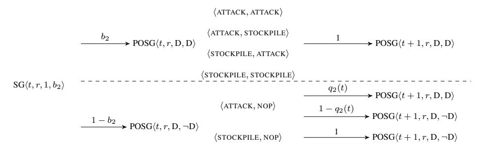
SGt, r, 1, b2 POSGt, r, D, ¬D POSGt, r, D, D POSGt + 1, r, D, D POSGt + 1, r, D, ¬D POSGt + 1, r, D, ¬D POSGt + 1, r, D, D ATTACK, ATTACK ATTACK, STOCKPILE STOCKPILE, ATTACK STOCKPILE, STOCKPILE ATTACK, NOP STOCKPILE, NOP b2 1 − b² 1 1 1 − q2(t) q2(t) Fig. 5: The relationship between the SG and the POSG models after disclose a vulnerability. SG-· denotes the game state of the SG model and POSG-· denotes the game state of the POSG model. Suppose player 1 discloses a vulnerability. Input : t: The index of the current round b1, b2: The probability that player 1 and player 2 have discovered the vulnerability. Output : NES(t, ∅, b1, b2)[i]: The utility of player i under the Nash equilibrium at round t before disclosure. ¹ if t >= MAXt then ² Game is over. ³ end ⁴ θ^S ← t, ∅, b1, b2; ⁵ Θ^T ← set of possible states transiting from θS; ⁶ max ← −∞; ⁷ foreach a^{S 1} ∈ A^S do ⁸ min ← ∞; ⁹ foreach a^{S 2} ∈ A^S do ¹⁰ t ← R(θS, a^{S 1} , a^{S 2} ) + ^θ∈Θ^S ΦS(θS, a^{S 1} , a^{S 2} )[θ]NES(θ); ¹¹ if min > t then ¹² min ← t; ¹³ end ¹⁴ end ¹⁵ if max < min then ¹⁶ max ← min; ¹⁷ end ¹⁸ end ¹⁹ NES(t, ∅, b1, b2)[1] ← max; ²⁰ NES(t, ∅, b1, b2)[2] ← -max; ²¹ return NES(t, b1, b2); Algorithm 1: The before-disclosure game algorithm. players have generated the exploit, then both of them should attack. If not, the player who did not disclose the vulnerability should attack once he has generated the exploit. The other player who disclosed the vulnerability should choose between attack and stockpile depending on the sum of the utilities at the current round and that in the future. VI. EVALUATION AND CASE STUDIES In this section, we apply our algorithm to calculate the Nash equilibrium of cyber-warfare games and discuss the following questions: The Attack-or-Disclose Question. Previous models [3, 10, 25, 31] limit that a player is allowed to choose only one action which is either attack or disclose. We extend to allow players playing a sequence of actions. Will a player get more utility if he is allowed to play a sequence of actions? The One-Must-Attack Question. The cyber-hawk model [25] concludes that at least one player will attack. Input : t: The index of the current round r: The index of the round at which a vulnerability is disclosed b1, b2: The probability that player 1 and player 2 have discovered the vulnerability. Output : NES(t, r, b1, b2): The player utility under the Nash equilibrium at round t after the vulnerability is disclosed at round r. ¹ if t >= MAXt then ² Game is over. ³ end ⁴ foreach i ∈ {1, 2} do ⁵ if bⁱ < 1 and t > r + δⁱ then ⁶ bⁱ ← 1; ⁷ end ⁸ end ⁹ if b¹ == 1 && b² == 1 then ¹⁰ NES(t, r, b1, b2) ← NE^P (t, r, D, D); ¹¹ end ¹² else if b² < 1 then ¹³ NES t, r, b1, b2 ← maxa^{P 1} ∈{ATTACK,STOCKPILE} b² · NE^P t, r, D, D + (1 − b2) · NE^P t, r, D, ¬D ; ¹⁴ end ¹⁵ else ¹⁶ NES t, r, b1, b2 ← mina^{P 2} ∈{ATTACK,STOCKPILE} b¹ · NE^P t, r, D, D + (1 − b1) · NE^P t, r, ¬D, D ; ¹⁷ end ¹⁸ return NES(t, r, b1, b2); Algorithm 2: The after-disclosure game algorithm. Does our model support this conclusion? If not, is there any counter-example? What causes the counter-example? The CGC Case Study. How to apply the model to published cyber-conflict events such as the Cyber Grand Challenge, which is a well-designed competition approximating a real-world scenario? Does our model improve the competitor's score if the other players do not change their actions in the game? The MAX^t Effect Evaluation. How does the configuration of MAX^t affect the results? Performance Evaluation. What is the runtime performance of the automatic strategic decision-making tool? We investigate the questions by performing several case studies. Although these cases have concrete parameter values, they characterize general situations in cyber warfare where players have different levels in one or more technical skills. The Attack-or-Disclose Question. Previous models assert that a player should either always attack, or always disclose. 16

Player 1 Player 2 pi(t) p1(t)=0.5, ∀t p2(t)=0.5, ∀t ui(t) u1(t)=1, ∀t u2(t) = 20, ∀t qi(t) q1(t)=0.2, ∀t q2(t)=0.9, ∀t δi δ¹ = 20 δ² = 20 hi(t) h1(t)=1 − 0.9t,t< 2 h2(t)=1 − 0.1t,t< 10 h1(t)=1, t ≥ 10 h2(t)=1, t ≥ 10 TABLE IV: Case I. Player 1's best strategy is to disclose then attack. However, using our tool, we find cases where a player has a better strategy than to attack or to disclose all the time. For example, consider a game with the parameters in Table IV. In this case, player 1's optimal strategy is to disclose and then attack 2 rounds after disclosure. Intuitively, there are three reasons for player 1 to choose the disclose-then-attack strategy. First, player 1 has more vulnerable resources than player 2, so he will lose if both players attack before disclosure. Second, player 2 has a relatively high ricochet probability, so he will be very likely to generate ricochet attacks if player 1 attacks. Finally, player 1 patches faster than player 2, so he will finish patching earlier, when player 2 is still partially vulnerable. Therefore, player 1 prefers disclose-then-attack strategy over only attacking or only disclosing. The One-Must-Attack Question. Previous work concludes that at least one player must attack [25]. However, we argue that the conclusion is inaccurate, by showing cases in which neither player prefers attacking. Consider the game with the settings shown in Table V. We find that both players will choose to PATCH after they find the vulnerability. The intuition is that player 1 should never choose to ATTACK because he will suffer a greater loss if player 2 launches ricochet attacks. Player 1 should also never choose to STOCKPILE, because player 2 may re-discover the vulnerability and then ATTACK. Therefore, player 1's best strategy is to PATCH once he discovers the vulnerability. After player 1 discloses a vulnerability, player 2 receives the patch and generates exploits based on the patch, which costs him δ² rounds. Within the rounds, player 1 would have completely patched his own machines, which makes any future attack from player 2 valueless. Furthermore, we observe two necessary elements leading to players' not attacking strategy: ricochet capability and patching capability. To illustrate our observation, we computed the Nash equilibrium of two other games, where we only changed the value of the ricochet or patching parameters, and we found that one player will prefer attacking in new games. First, we consider the scenario excluding ricochet. We keep the parameters Table V, but set qi(t)=0, ∀t. We observe that both players will attack until the end of the game. Because ATTACK always bring positive benefit while STOCKPILEand NOP always bring 0 benefit, ATTACK dominates STOCKPILEand NOP at any round. Therefore, the optimal strategy for both players is to attack as soon as they discover the vulnerability. Second, we consider the scenario where one player slows down his patching speed. Suppose we replace the original patching function h2(t) with h2(t)=1 − 0.1^t ,t < 20 and h2(t)=1, t ≥ 20. We observe that the best strategy for player 1 is to attack, since some of the player 2's resources remain Player 1 Player 2 pi(t) p1(t)=0.8, ∀t p2(t)=0.01, ∀t ui(t) u1(t)=2, ∀t u2(t) = 20, ∀t qi(t) q1(t)=0.2, ∀t q2(t)=0.9, ∀t δi δ¹ = 20 δ² = 20 hi(t) h1(t)=1 − 0.9t,t< 10 h2(t)=1 − 0.1t,t< 10 h1(t)=1, t ≥ 10 h2(t)=1, t ≥ 10 TABLE V: Case II. Both players' best strategy is to disclose without attacking. vulnerable after player 1 is done with patching. This case indicates that even though the ricochet attack exists, if a player does not patch fast enough, he will still be attacked by his opponent. In conclusion, we find that both ricochet and speedy patching are necessary in order to prevent adversaries from attacking. The CGC Case Study. The Cyber Grand Challenge (CGC) is an automated cyber-security competition designed to mirror "real-world challenges" [12]. This competition provides an excellent opportunity to evaluate the strategies suggested by our model against those actually carried out by competitors. The CGC final consists of 95 rounds. In this case study, we experimented on the ranking of the third-place team in the Cyber Grand Challenge, Shellphish. Based on their public discussions regarding their strategy, Shellphish simply attacked and patched right away [13]. This made them an optimal subject of this case study, as, since they would use their exploits as soon as possible (rather than stockpiling them), we can closely estimate their technical acumen for the purposes of testing our model. We call our modified, more strategic, player "Strategic-Shellphish". In our experiment, we adapted our model to the CGC final in the following way. First, we update the reward function on the CGC scoring mechanism. As the CGC final is not a zero-sum game, we compute the Nash equilibrium by focusing on the current round. Second, we separate the game by binaries, and for each binary we model Strategic-Shellphish as one player while all the non-Shellphish team as the other player. Third, we estimated the game parameters according to the data from the earlier rounds, then calculated the optimal strategy and applied the strategy in the later rounds. For example, we get the availability score for the patch by deploying it in the earlier rounds. The data is from the public release from DARPA, which includes the player scores for each vulnerable binaries in each round. In the first CGC experiment, we estimated the game parameters by the information of the first 80 rounds of the game, and applied the model on the 80-95 rounds. This range included 11 challenge binaries, and we simulated Shellphish's performance, if they had used our model for strategy determinations, across these programs. The score comparison for each vulnerability is shown in Figure 6, with the x axis representing the 11 binaries and the y axis representing the scores. The new scores are either higher or equal to the original score. Among these binaries, our model helps improve 5 cases out of 11. The overall score for the 11 vulnerabilities is shown in Figure 7. The original Shellphish team got 38598.7 points, while our model got 40733.3 points. 17

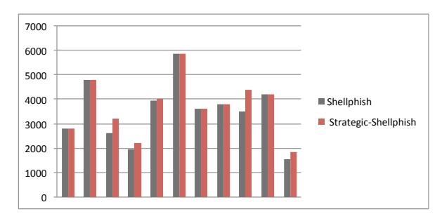
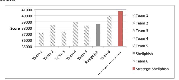
• -- Fig. 6: The per-vulnerability score comparison between the original Shellphish team and Strategic-Shellphish – the Shellphish team + our model. - - - - - Fig. 7: The overall score comparison between the original Shellphish team and Strategic-Shellphish for the game round 80-95. Moreover, our Strategic-Shellphish team won against all other teams in terms of these 11 vulnerabilities. We observed that Strategic-Shellphish withdrew the patch of some vulnerabilities after the first round of patching. After the first round of patching, Strategic-Shellphish got the precise score for availability, and this helped it compare the cost of patching to the expected lost in the future rounds. In the second CGC experiment, we estimated the game parameters by the information of the first 15 rounds. Given the parameters, Strategic-Shellphish calculates the likelihood that the other teams discovers the vulnerability, and it uses our algorithm to determine the best response. Before it is wellaware of the patching cost, we assigned the cost to 0. After the first round of patching, we updated the patching cost and adjusted the future strategy. The score for the entire game is shown in Figure 8. The original Shellphish team got 254,452 points and ranked third in the game. On the other hand, the Strategic-Shellphish got 268,543 points, which is 6000 points higher than the score of the original 2nd-rank team. Our experiment highlights the importance of our model as well as the optional strategy solution. If a team such like Shellphish used our model, it could have achieved a better result compared to its original strategy. In fact, in the Cyber Grand Challenge, the difference between third (Shellphish) and second (Strategic-Shellphish) place was $250,000. The MAX^t Effect Evaluation. To understand the effect of MAX^t on the final result, we fixed the parameter values in Table IV and varied the value of MAX^t from 1 to 15. For each game, we computed the Nash equilibrium and its corresponding players' utilities. 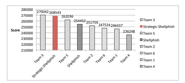As the game is a zero-sum game and the utility of player 2 is always symmetric to that of player 1, we - - - - - - Fig. 8: The overall score comparison between the original Shellphish team and Strategic-Shellphish for the entire game. will focus on player 1's utility. 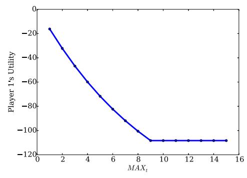Fig. 9: Player 1's Utility over different maximum number of round (MAXt). Figure 9 shows player 1's utility. We observed that when MAX^t is small, the change of MAX^t will affect the Nash equilibrium and players' utilities. As MAX^t becomes larger, the change of MAX^t will no longer affect the Nash equilibrium, and the players' utilities will become stable. In our case, when MAX^t = 1, player 1 will patch and player 2 will attack for both rounds. When MAX^t = 2, player 1 will disclose at the first round and attack at the second round, while player 2 will attack for both rounds, and, meanwhile, patch if player 1 discloses the vulnerability. When MAX^t ≥ 3, player 1 will disclose at the first round and attack since the third round. This observation implies that players tend to be more aggressive in a shorter game. It also explains why the result of the cyberhawk model [25] is suboptimal: if the game is considered as a single-round game, players will neglect the loss in the future and make a local optimal strategy rather than a global optimal one. Performance Evaluation. In this evaluation, we fixed the player parameters and measured the time for computing the Nash equilibrium under different MAX^t values from 1 to 50. We show the time performance in Figure 10. Based on the figure, we found that although the time of computing increases as MAX^t grows, our tool is able to find the Nash equilibrium of all games within seconds. In practical, MAX^t needs to be configured properly in order to balance between the action frequency (i.e. Should a player act per minutes or per day?) and the action performance (i.e. How long do we need to respond to the zero-day vulnerability events?). 18

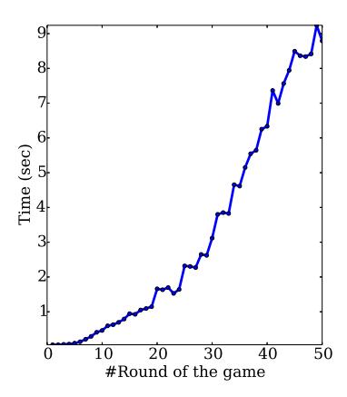
Fig. 10: The time (in second) for computing the Nash equilibrium over different maximum number of round MAXt. VII. DISCUSSION AND FUTURE WORK Our work advances zero-day strategy research by constructing a game model covering features that are of great significance in real-world cyber warfare, such as activity over multiple rounds, partial availability of information, and emergent offensive techniques like APEG and ricochet. In this section, we discuss some aspects to be addressed in future work. Irrational Players and Collusion. We focus on a setting with rational players engaged in zero-sum games. It is well established that governments and people act irrational from time to time. Nonetheless, an analysis of rational behavior highlights an important consideration point. We leave the modeling of non-rational behavior and non-zero-sum games as future work. Parameter Sensitivity. Our model employs parameters to capture players' different skill levels. These parameters need to be evaluated, and one way is to use a relevant benchmark proposed by Axelrod et al. [3]. For example, one can estimate pi(t) by reasoning about the ratio of the vulnerabilities independently rediscovered in software from the research by Bilge et al. [5]. As the White House stated that the government weighed the likelihood that the other nations re-discover the vulnerability, the evaluation approach should have already existed. In the future, we need to investigate the robustness of the model under different parameter margins. Multiple Nash Equilibria. It is possible that multiple Nash equilibria exist in a cyber-warfare game. However, due to the zero-sum game property, player utilities remain the same for all Nash equilibria. Therefore, any Nash equilibrium is players' optimal strategy. Although we do not discuss the entire set of possible Nash equilibria, finding them all is a straightforward extension of our algorithm, in the way that one could record all strategies with same value as the maximum one. Deception. Although the game parameters are public, they can be manipulated by players. For example, a player could pretend to be weak in generating exploits by never launching any attack against anyone. In our paper, we do not consider player deception, and we leave it for future work. Inferring Game State from Parameters. We consider that players infer the states of other players by detecting attacks or learning vulnerability disclosure. However, we do not consider that players could these state by reasoning about game parameters. For example, suppose we have a game with public game parameters denoting that player 1 is able to capture all the attacks and player 2 should always attack after he generates an exploit. In this case, if player 1 does not detect attacks from player 2, then player 2 has not generated an exploit, and the belief on player 2 should be zero all the time until player 1 detects an attack. To tackle this problem, a possible way is to solve the game separately with different groups of parameter conditions. Multiple Vulnerabilities. Our game model focuses on one vulnerability. We assume that vulnerabilities are independent, and a game with multiple vulnerabilities can be viewed as separate games each of which has a single vulnerability. To combine multiple vulnerabilities in a game, a possible direction is to consider modification of the game parameters. For example, instead of the probability that the opponent rediscovers the vulnerability, we could use the probability that the opponent discovers any vulnerabilities. Also, we could extend the utility function by including the utility gained from other vulnerabilities. Limited Resources. When players are constrained by limited resources, they may have fewer strategy choices. For example, if a player has limited resources, he may not be able to simultaneously generate an exploit and generate a patch. The limited resources may affect players' best response as well as the Nash equilibrium. In the future, we need to come up with updated model and algorithm to address this issue. The Incentives of Patching. In our model, we consider patching as a defensive mechanism that only prevents players from losing utility. This leads to players not having incentives to disclose a vulnerability. We argue that patching might bring positive benefits to players. For instance, a player would have a better reputation if he chooses to disclose a vulnerability and patch their machines. We leave the consideration of the positive reputation caused by disclosure as future work. VIII. CONCLUSION In this paper, we present a cyber-warfare model which considers strategies over time, addresses players' uncertainty about their opponents, and accounts for new offensive and defensive techniques that can be employed for cyber-warfare, e.g., the ricochet attack and APEG. We propose algorithms for computing the Nash equilibrium of the model, and our algorithm is able to find better strategies than previous work within seconds. Moreover, by solving the game model, we allow decision makers to calculate utility in scenarios like patch-then-exploit, as well as show where, in the parameter space of the game model, it makes more sense to patch than to attack. Our model also challenges previous results, which conclude that at least one player should attack, by showing scenarios where attacking is not optimal for either player. 19

IX. ACKNOWLEDGEMENTS The authors would like to thank our shepherd, Jeremiah M. Blocki, and the reviewers for the valuable suggestions. We would also like to thank Vyas Sekar for his comments on the project. REFERENCES [1] R. Anderson and T. Moore. The economics of information security. Science (New York, N.Y.), 314(2006):610–613, 2006. [2] G. Ateniese, B. Magri, and D. Venturi. Subversionresilient signature schemes. In Proceedings of the 22nd ACM SIGSAC Conference on Computer and Communications Security, pages 364–375, 2015. [3] R. Axelrod and R. Iliev. Timing of cyber conflict. Proceedings of the National Academy of Sciences, 111(4):1298– 1303, 2014. [4] T. Bao, R. Wang, Y. Shoshitaishvili, and D. Brumley. Your Exploit is Mine: Automatic Shellcode Transplant for Remote Exploits. In Proceedings of the 38th IEEE Symposium on Security and Privacy, 2017. [5] L. Bilge and T. Dumitras. Before we knew it—an empirical study of zero-day attacks in the real world. In Proceedings of the 2012 ACM Conference on Computer and Communications Security, pages 833–844. ACM, 2012. [6] D. Brumley, P. Poosankam, D. Song, and J. Zheng. Automatic patch-based exploit generation is possible: Techniques and implications. In Proceedings of the 2008 IEEE Symposium on Security and Privacy, pages 143–157. IEEE, 2008. [7] H. Cavusoglu, H. Cavusoglu, and S. Raghunathan. Emerging issues in responsible vulnerability disclosure. Fourth Workshop on the Economics of Information Security, pages 1–31, 2005. [8] R. A. Clarke and R. K. Knake. Cyber War: The Next Threat to National Security and What to Do About It. HarperCollins, 2010. [9] M. Costa, J. Crowcroft, M. Castro, A. Rowstron, L. Zhou, L. Zhang, and P. Barham. Vigilante: End-to-end containment of internet worms. In Proceedings of the 20th ACM Symposium on Operating Systems Principles, pages 133–147. ACM, 2005. [10] C. Czosseck and K. Podins. A vulnerability-based model of cyber weapons and its implications for cyber conflict. International Journal of Cyber Warfare and Terrorism, 2(1):14–26, 2012. [11] M. Daniel. Heartbleed: Understanding when we disclose cyber vulnerabilities. http://www.whitehouse.gov/blog/2014/04/28/heartbleedunderstanding-when-we-disclose-cyber-vulnerabilities, 2014. [12] DARPA. CGC frequently asked questions. https://cgc. darpa.mil/CGC_FAQ.pdf. [13] DARPA. DARPA's Cyber Grand Challenge: Final event program. https://www.youtube.com/watch?v= n0kn4mDXY6I. [14] C. Daskalakis, P. W. Goldberg, and C. H. Papadimitriou. The complexity of computing a Nash equilibrium. Society for Industrial and Applied Mathematics, 39(1):195–259, 2009. [15] L. M. Dermed and C. L. Isbell. Solving stochastic games. In Annual Conference on Neural Information Processing Systems, pages 1186–1194, 2009. [16] J. Franklin, V. Paxson, A. Perrig, and S. Savage. An inquiry into the nature and causes of the wealth of Internet miscreants. In Proceedings of the 14th ACM Conference on Computer and Communications Security, pages 375– 388, 2007. [17] B. Fung. The NSA hacks other countries by buying millions of dollars' worth of computer vulnerabilities. https://www.washingtonpost.com/news/the-switch/wp/ 2013/08/31/the-nsa-hacks-other-countries-by-buyingmillions-of-dollars-worth-of-computer-vulnerabilities/, 2013. [18] A. Greenburgh. Kevin Mitnick, once the world's most wanted hacker, is now selling zero-day exploits. https://www.wired.com/2014/09/kevin-mitnickselling-zero-day-exploits/, 2014. [19] J. Grossklags. An empirical study of web vulnerability discovery ecosystems. In Proceedings of the 22nd ACM SIGSAC Conference on Computer and Communications Security, pages 1105–1117, 2015. [20] K. Leyton-Brown and Y. Shoham. Essentials of Game Theory: A Concise Multidisciplinary Introduction. 2008. [21] Y. Luo, F. Szidarovszky, Y. Al-Nashif, and S. Hariri. Game theory based network security. Journal of Information Security, 1:41–44, 2010. [22] K. Lye and J. M. Wing. Game strategies in network security. International Journal of Information Security, 4(1-2):71–86, 2005. [23] L. MacDermed, C. L. Isbell, and L. Weiss. Markov games of incomplete information for multi-agent reinforcement learning. In Workshops at the Twenty-Fifth AAAI Conference on Artificial Intelligence, pages 43–51, 2011. [24] M. H. Manshaei, Q. Zhu, T. Alpcan, T. Bac¸sar, and J.-P. Hubaux. Game theory meets network security and privacy. ACM Computing Surveys, 45(3):1–39, 2013. [25] T. Moore, A. Friedman, and A. D. Procaccia. Would a 'cyber warrior' protect us? Exploring trade-offs between attack and defense of information systems. In Proceedings of the Workshop on New Security Paradigms, pages 85–94, 2010. [26] J. F. Nash. Equilibrium points in n-person games. Proceedings of the National Academy of Sciences of the United States of America, 36(1):48–49, 1950. [27] N. Perlroth and D. E. Sanger. Nations buying as hackers sell flaws in computer code. http: //www.nytimes.com/2013/07/14/world/europe/nationsbuying-as-hackers-sell-computer-flaws.html?_r=0, 2013. [28] N. Robert Joyce. Disrupting nation state actors. https: //www.youtube.com/watch?v=bDJb8WOJYdA. 20

[29] S. Roy, C. Ellis, S. Shiva, D. Dasgupta, V. Shandilya, and Q. Wu. A survey of game theory as applied to network security. In Proceedings of the 43rd Hawaii International Conference on System Sciences, pages 1–10. IEEE, 2010. [30] Samurai CTF Team. We are Samurai CTF and we won Defcon CTF this year. AMA! http://www.reddit.com/r/netsec/comments/y0nnu/we_ are_samurai_ctf_and_we_won_defcon_ctf_this/c5r9osm, 2013. [31] H. C. Schramm, D. L. Alderson, W. M. Carlyle, and N. B. Dimitrov. A game theoretic model of strategic conflict in cyberspace. Military Operations Research, 19(1):5–17, 2014. [32] L. S. Shapley. Stochastic games. Proceedings of the National Academy of Sciences, 39(10):1095, 1953. [33] Y. Shoham and K. Leyton-brown. Multiagent Systems: Algorithmic, Game-Theoretic, and Logical Foundations. Cambridge University Press, 2009. [34] B. Stock, S. Pfistner, B. Kaiser, S. Lekies, and M. Johns. From facepalm to brain bender: Exploring client-side cross-site scripting categories and subject descriptors. In Proceedings of the 22nd ACM SIGSAC Conference on Computer and Communications Security, pages 1419– 1430, 2015. [35] M. Tambe, M. Jain, J. A. Pita, and A. X. Jiang. Game theory for security: Key algorithmic principles, deployed systems, lessons learned. In Proceedings of the 50th Annual Allerton Conference on Communication, Control, and Computing, pages 1822–1829. IEEE, 2012. [36] K. Zetter. US used zero-day exploits before it had policies for them. http://www.wired.com/2015/03/us-used-zeroday-exploits-policies/, 2015. [37] L. Zettlemoyer, B. Milch, and L. Kaelbling. Multi-agent filtering with infinitely nested beliefs. In Advances in Neural Information Processing Systems, pages 1–8, 2009. 21